Load Packages
First I need to load up the packages I’ll need
library(sf)
library(ggplot2) #development version!
## devtools::install_github("tidyverse/ggplot2")
library(tidyverse)
library(readr)
library(cowplot)
library(sp)
library(gridExtra)
library(plyr)
library(dplyr)
library(ggrepel)
Import Postcode Data
Now I import my data. I filter for the Arran postcodes, (since Arran all begins ‘KA27’). (I’ve already downloaded it but you can use the below download code). temp <- tempfile() download.file(“https://www.freemaptools.com/download/full-postcodes/ukpostcodes.zip”,temp) ukpostcodes <- read.csv(unz(temp, “ukpostcodes.csv”)) unlink(temp)
#Add download commands for data.
## Finding the Arran coordinates
arrancoordinates <- read.csv("../alldata/ukpostcodes.csv") %>%
 filter(substr(postcode,1,4)=="KA27")

#Find way to replace with existing SIMD shape files
arransubsect <- read_sf("../alldata/Scotland_pcs_2011") %>%
filter(substr(label,1,4)=="KA27")
Import SIMD data
Now I load the SIMD data, containing the geometries (shapefiles) and SIMD data (percentiles, etc) (Can be downloaded from the below addresses). http://sedsh127.sedsh.gov.uk/Atom_data/ScotGov/ZippedShapefiles/SG_SIMD_2016.zip http://sedsh127.sedsh.gov.uk/Atom_data/ScotGov/ZippedShapefiles/SG_SIMD_2012.zip http://sedsh127.sedsh.gov.uk/Atom_data/ScotGov/ZippedShapefiles/SG_SIMD_2009.zip http://sedsh127.sedsh.gov.uk/Atom_data/ScotGov/ZippedShapefiles/SG_SIMD_2006.zip http://sedsh127.sedsh.gov.uk/Atom_data/ScotGov/ZippedShapefiles/SG_SIMD_2004.zip
temp <- tempfile() download.file(“http://sedsh127.sedsh.gov.uk/Atom_data/ScotGov/ZippedShapefiles/SG_SIMD_2016.zip”,temp) arran2016 <- read_sf(unz(temp, “SG_SIMD_2016”))[c(4672,4666,4669,4671,4667,4668,4670),] %>% slice(match(reorderedvector, DataZone)) unlink(temp)
reorderedvector<- c("S01011174", "S01011171", "S01011177", "S01011176", "S01011175", "S01011173", "S01011172" )

arran2016 <- read_sf("../alldata/SG_SIMD_2016")[c(4672,4666,4669,4671,4667,4668,4670),] %>%
  slice(match(reorderedvector, DataZone))

Arrandz2012 <- c(4409,4372,4353,4352,4351,4350,4349)

arran2012 <- read_sf("../alldata/SG_SIMD_2012")[Arrandz2012,]
arran2009 <- read_sf("../alldata/SG_SIMD_2009")[Arrandz2012,]
arran2006 <- read_sf("../alldata/SG_SIMD_2006")[Arrandz2012,]
arran2004 <- read_sf("../alldata/SG_SIMD_2004")[Arrandz2012,]

sharedvariables <- intersect(colnames(arran2016), colnames(arran2012)) %>%
  intersect(colnames(arran2009))  %>%
  intersect(colnames(arran2006))  %>%
  intersect(colnames(arran2004))

arran20162 <- arran2016 %>%
  select(sharedvariables) %>%
  mutate(year="2016")
arran20122 <- arran2012 %>%
  select(sharedvariables) %>%
  mutate(year="2012")
arran20092 <- arran2009 %>%
  select(sharedvariables) %>%
  mutate(year="2009")
arran20062 <- arran2006 %>%
  select(sharedvariables) %>%
  mutate(year="2006")
arran20042 <- arran2004 %>%
  select(sharedvariables) %>%
  mutate(year="2004")

arransimd <- rbind(arran20162,arran20122,arran20092,arran20062,arran20042) %>%
mutate(
    lon = map_dbl(geometry, ~st_centroid(.x)[[1]]),
    lat = map_dbl(geometry, ~st_centroid(.x)[[2]])
    )

arransimd$listID <- revalue(arransimd$DataZone,
               c("S01004409"="S01004409/S01011174", "S01004372"="S01004372/S01011171", "S01004353"="S01004353/S01011177", "S01004352"="S01004352/S01011176", "S01004351"="S01004351/S01011175", "S01004350"="S01004350/S01011173", "S01004349"="S01004349/S01011172", "S01011174"="S01004409/S01011174", "S01011171"="S01004372/S01011171", "S01011177"="S01004353/S01011177", "S01011176"="S01004352/S01011176", "S01011175"="S01004351/S01011175", "S01011173"="S01004350/S01011173", "S01011172"="S01004349/S01011172"))
Initial Plots
The reason I’ve downloaded all the DataZones shapefiles individually is because they change between 2016 and 2012. See the small differences.
rbind(arran20162,arran20122) %>%
  ggplot() +
  geom_sf(aes(fill = DataZone)) +
  facet_wrap('year') +
  theme_grey() +
  theme(legend.position="none") +
  theme(axis.text.x=element_text(angle=45, hjust = 1))
Arran SIMD Health Percentiles
Now I want to look at percentile data.
arransimd %>%
filter(listID == unique(arransimd$listID))  %>%
  ggplot() +
  geom_sf(aes(fill = Percentile)) +
  facet_wrap('year', nrow=1) +
  theme_grey() +
  geom_text(aes(label = Percentile, x = lon, y = lat), size = 2, colour = "white") +
  theme(axis.text.x=element_blank(),
        axis.ticks.x=element_blank(),
        axis.text.y=element_blank(),
        axis.ticks.y=element_blank(),
        axis.title.x = element_blank(),
        axis.title.y = element_blank()) +
theme(legend.position="bottom") 
There we are. The SIMD health percentiles of Arran zones throughout SIMD history. And I’ve learned a little bit about graphics in R.
See this image at a larger size.
Now I want to overlay the postcodes by Datazone. To do this I’ve converted both the Arran coordinates and Arran (2016) shapefiles into spatial points/polygons, converted them into a common CRS, and then compared them by using ‘plyr::over()’. This gives me the object ‘namingdzpostcode’, with the postcode rows grouped into IDs (unidentified datazones).
simple.sf <- st_as_sf(arrancoordinates, coords=c('longitude','latitude'))
st_crs(simple.sf) <- 4326

exampleshapes <- sf:::as_Spatial(arran2016$geometry) %>%
  spTransform(CRS("+proj=longlat +datum=WGS84"))

examplepoints <- sf:::as_Spatial(simple.sf$geom) %>%
  spTransform(CRS("+proj=longlat +datum=WGS84"))

namingdzpostcode <- over(exampleshapes, examplepoints, returnList = TRUE)
I can then take a member reference from the orginal postcode list, which gives me a selection of the rows in that DZ. For simplicity I’ve written this as a new function.
Mutate arrancoordinates to label the IDs
function100 <- function(argument)
{
  argument <- arrancoordinates[namingdzpostcode[[argument]],] %>% mutate(DataZone=argument)
}

arrancoordinates <- lapply(1:7,function100)
arrancoordinates <- rbind(arrancoordinates[[1]], arrancoordinates[[2]], arrancoordinates[[3]], arrancoordinates[[4]], arrancoordinates[[5]], arrancoordinates[[6]], arrancoordinates[[7]])

arrancoordinates$listID <- revalue(as.character(arrancoordinates$DataZone),
               c('1'="S01004409/S01011174", '2'="S01004372/S01011171", '3'="S01004353/S01011177", '4'="S01004352/S01011176", '5'="S01004351/S01011175", '6'="S01004350/S01011173", '7'="S01004349/S01011172"))
Labelling the namingdzpostcode list
names(namingdzpostcode) <- c(unique(arransimd$listID))Subsecting the coordinates
coordinateexample <- arrancoordinates %>%
  select(postcode, latitude, longitude, listID) %>%
  filter(listID == unique(arrancoordinates$listID)[1])
Individual Datazones
filter(arransimd, year == 2016) %>%
  ggplot() +
  theme_grey() +
  theme(axis.text.x=element_blank(),
        axis.ticks.x=element_blank()) +
  theme(legend.position="none") +
  facet_wrap('listID', nrow = 1) +
  geom_sf(aes(fill = DataZone))
Plotting DataZones by facet_grid
arransimd %>%
ggplot() +
  geom_sf(aes(fill = Percentile)) +
  facet_grid(listID ~ year) +
  theme_grey() +
  geom_text(aes(label = Percentile, x = lon, y = lat), size = 2, colour = "white") +
  theme(axis.text.x=element_blank(),
        axis.ticks.x=element_blank(),
        axis.title.x = element_blank(),
        axis.title.y = element_blank()) +
  theme(legend.position="bottom")
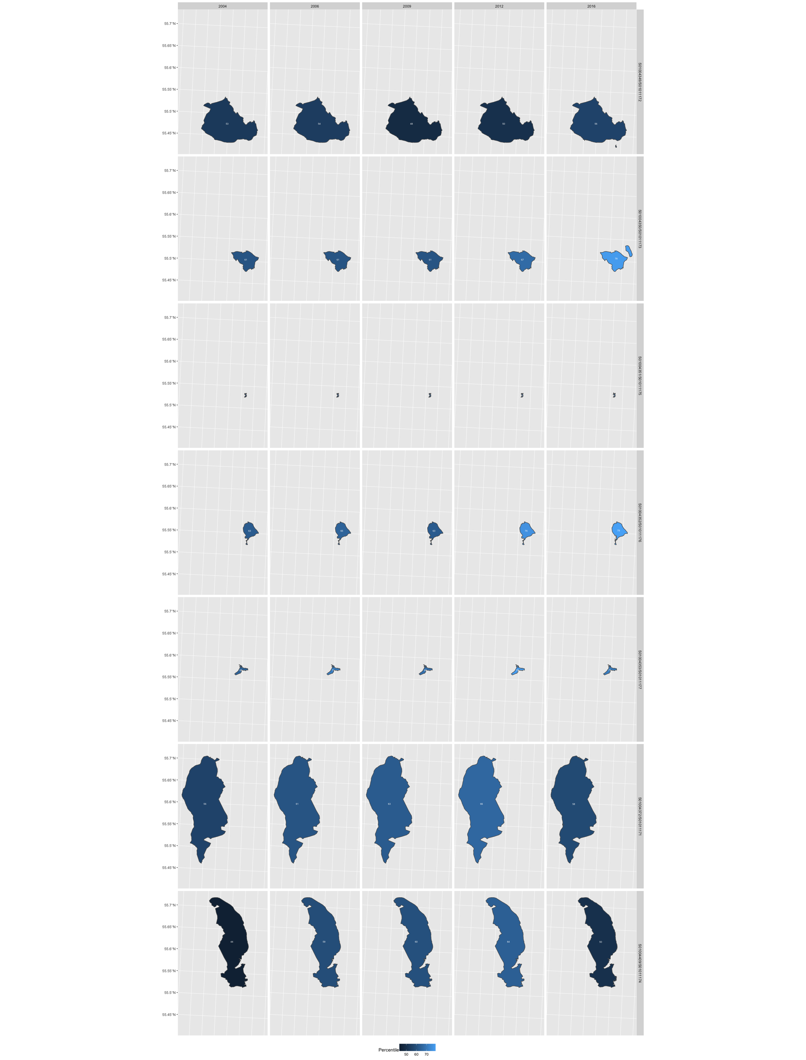
Postcodes overlayed onto datazone.
ggplot() +
  geom_sf(data=arransimd) +
  geom_point(data=arrancoordinates,
             mapping = aes(x = longitude, y = latitude),
             size=1) +
  theme_grey() +
  theme(axis.title.x = element_blank(),
        axis.title.y = element_blank(),
        axis.text.x=element_blank(),
        axis.ticks.x=element_blank()) +
  coord_sf(crs= 4326, datum = sf::st_crs(4326)) +
  facet_wrap('listID', nrow = 1)
See this plot at a larger scale.
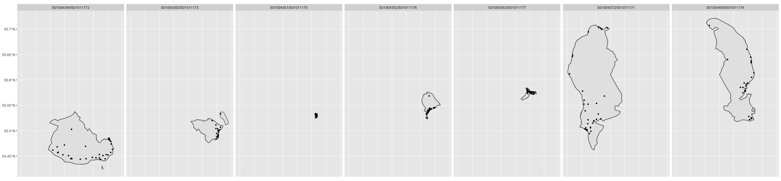
thisfunction2 <- function(argument)
{arransimd %>%
  filter(listID == argument)  %>%
  ggplot() +
  geom_sf() +
  theme_grey() +
  geom_point(data = filter(arrancoordinates, listID == argument),
             mapping = aes(x = longitude, y = latitude), size=1) +
  geom_text_repel(data = filter(arrancoordinates, listID == argument),
            aes(label = filter(arrancoordinates,
                               listID == argument)$postcode,
                x = longitude, y = latitude), size=2) +
  theme(axis.title.x = element_blank(),
        axis.title.y = element_blank(),
        axis.text.x=element_blank(),
        axis.ticks.x=element_blank(),
        axis.text.y=element_blank(),
        axis.ticks.y=element_blank()) +
  coord_sf(crs= 4326, datum = sf::st_crs(4326))
}

output2 <- lapply(unique(arransimd$listID), thisfunction2)
grid.arrange(output2[[1]], output2[[2]], output2[[3]], output2[[4]], output2[[5]], output2[[6]], output2[[7]], ncol = 7)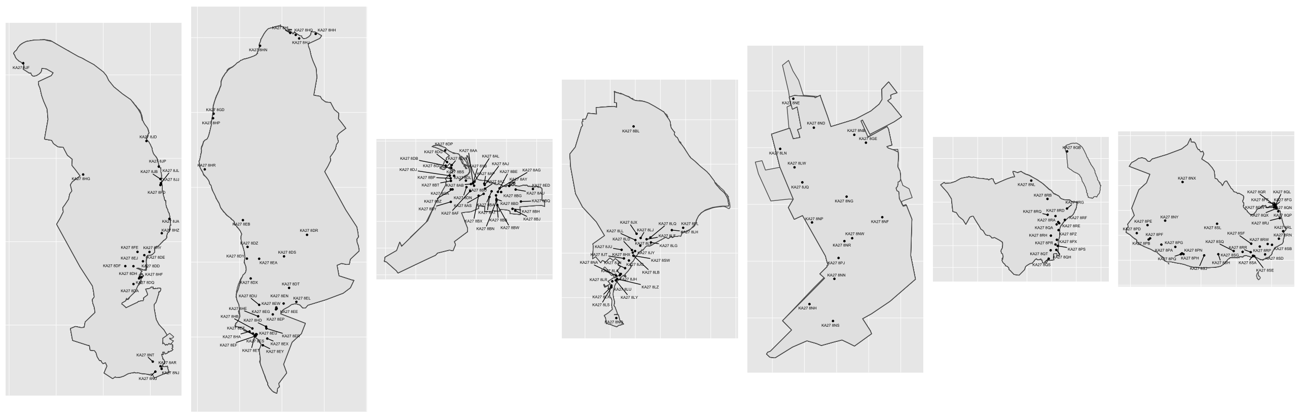
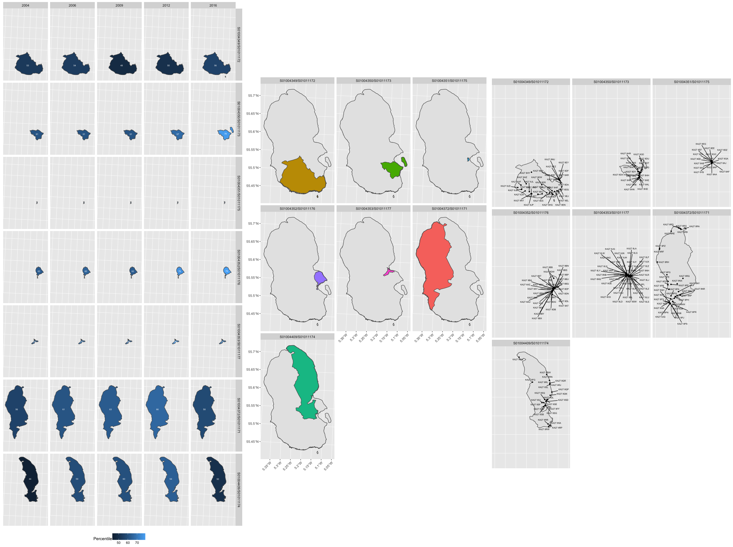
Plots
function10 <- function(argument)
{
a <- arransimd %>%
mutate(
    lon = map_dbl(geometry, ~st_centroid(.x)[[1]]),
    lat = map_dbl(geometry, ~st_centroid(.x)[[2]])
    ) %>%
filter(listID == argument)  %>%
  ggplot() +
  geom_sf(aes(fill = Percentile)) +
  facet_wrap('year') +
  theme_grey() +
  geom_text(aes(label = Percentile, x = lon, y = lat), size = 2, colour = "white") +
  theme(axis.text.x=element_blank(),
        axis.ticks.x=element_blank(),
        axis.text.y=element_blank(),
        axis.ticks.y=element_blank(),
        axis.title.x = element_blank(),
        axis.title.y = element_blank()) +
  theme(legend.position="bottom") +
  scale_fill_continuous(limits = c(40,80))

b <- arransimd %>%
  filter(listID == argument)  %>%
  ggplot() +
  geom_sf(data = arransubsect) +
  theme_grey() +
  theme(axis.text.x=element_text(angle=45, hjust = 1)) +
  theme(legend.position="bottom") +
  geom_sf(aes(fill = DataZone))

c <- arransimd %>%
  filter(listID == argument)  %>%
  ggplot() +
  geom_sf() +
  theme_grey() +
  geom_point(data = filter(arrancoordinates, listID == argument),
             mapping = aes(x = longitude, y = latitude), size=1) +
  geom_text_repel(data = filter(arrancoordinates, listID == argument),
            aes(label = filter(arrancoordinates,
                               listID == argument)$postcode,
                x = longitude, y = latitude), size=2) +
  theme(axis.title.x = element_blank(),
        axis.title.y = element_blank(),
        axis.text.x=element_blank(),
        axis.ticks.x=element_blank(),
        axis.text.y=element_blank(),
        axis.ticks.y=element_blank()) +
  coord_sf(crs= 4326, datum = sf::st_crs(4326))

grid.arrange(a, b, c, nrow = 1)
}
See these plots at a larger scale.
a2 <- arransimd %>%
  ggplot() +
  geom_sf(aes(fill = Percentile)) +
  facet_grid(listID ~ year) +
  theme_grey() +
  geom_text(aes(label = Percentile, x = lon, y = lat), size = 2, colour = "white") +
  theme(axis.text.x=element_blank(),
        axis.ticks.x=element_blank(),
        axis.text.y=element_blank(),
        axis.ticks.y=element_blank(),
        axis.title.x = element_blank(),
        axis.title.y = element_blank()) +
  theme(legend.position="bottom")

b2 <- arransimd %>%
  filter(year == 2016)  %>%
  ggplot() +
  facet_wrap("listID") +
  geom_sf(data = arransubsect) +
  theme_grey() +
  theme(axis.text.x=element_text(angle=45, hjust = 1)) +
  theme(legend.position="none") +
  geom_sf(aes(fill = DataZone))

c2 <- arransimd %>%
 filter(year == 2016)  %>%
  ggplot() +
  facet_wrap("listID") +
  geom_sf() +
  theme_grey() +
  geom_point(data = arrancoordinates,
             mapping = aes(x = longitude, y = latitude), size=1) +
 geom_text_repel(data = arrancoordinates, aes(label = arrancoordinates$postcode,
                x = longitude, y = latitude), size=2) +
  theme(axis.title.x = element_blank(),
        axis.title.y = element_blank(),
        axis.text.x=element_blank(),
        axis.ticks.x=element_blank(),
        axis.text.y=element_blank(),
        axis.ticks.y=element_blank()) +
  coord_sf(crs= 4326, datum = sf::st_crs(4326))

grid.arrange(a2, b2, c2, ncol = 3)
See this plot at a larger scale.